Visualizing Rushing Offense Through Run Gap and Location Data
Bringing new perspective to rushing success rate with isomorphic data modeling
Intro!
Methodology
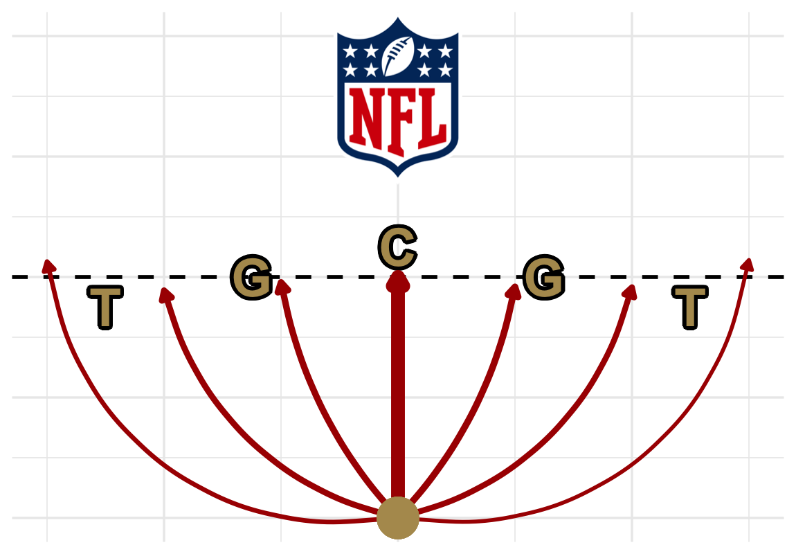
For all designed runs in the modern NFL, the rush gap and location utilized by the ball carrier is denoted in the play-by-play data record. The rush location signifies the direction of the field the ball carrier ran towards after receiving the handoff (left, right, or middle). The rush gap signifies the the direction the ball carrier ran in relative to the holes created by their offensive line. "End" rushes occur when the carrier goes around the outside of their tackle (the outermost bookends of an offensive line), "tackle" rushes exist in the gaps created between a tackle and a guard (the player between a tackle and the center), "guard" rushes exist in the gaps created between a guard and the center, and some rushes have gap denoted as NA which exclusively applies to rush directly up the middle of the field.
By creating a new variable run-location-gap as the pasted value of run gap and location and ordering relative to real-life position, we can divide
rush attempts by the path taken by the running back and analyze performance along those lines. Although any variety of performance metrics could be collected and grouped by location and gap,
I chose to measure by success rate, a metric that indicates the proportion of plays in a sample that bring the offense closer to scoring than they were before the play began, for the sake of
this exercise due to its stability. Other meaningful statistics that would have been adequate are EPA/rush, first downs/rush, and yards/rush [What are these metrics?]
The beauty of this project lies in the visualization, where I attempted to make the graph as isomorphic as possible to be used as an easy tool for understanding where a player or team is succeeding or struggling to run the football. Each arrow denotes a possible path for the rusher to take, and the endpoint of the arrow indicates the success rate for that gap and location, mirroring the "yardage" gained or lost by a ball carrier on a given play. Surrounding the paths is a mockup of an offensive line listed by position for physical reference. The thickness of each arrow is plotted relative to sample size, which shows the frequency at which players/teams target each possible path. The final visual added to the graph is a dashed baseline, set to a success rate of 0.40 (the rounded league average on designed rushes) for this implementation.
- Data Source: nflfastR package (2025 regular season data).
- Tools: dplyr for data processing, ggplot2 and nflplotR for visuals.
Results and Analysis
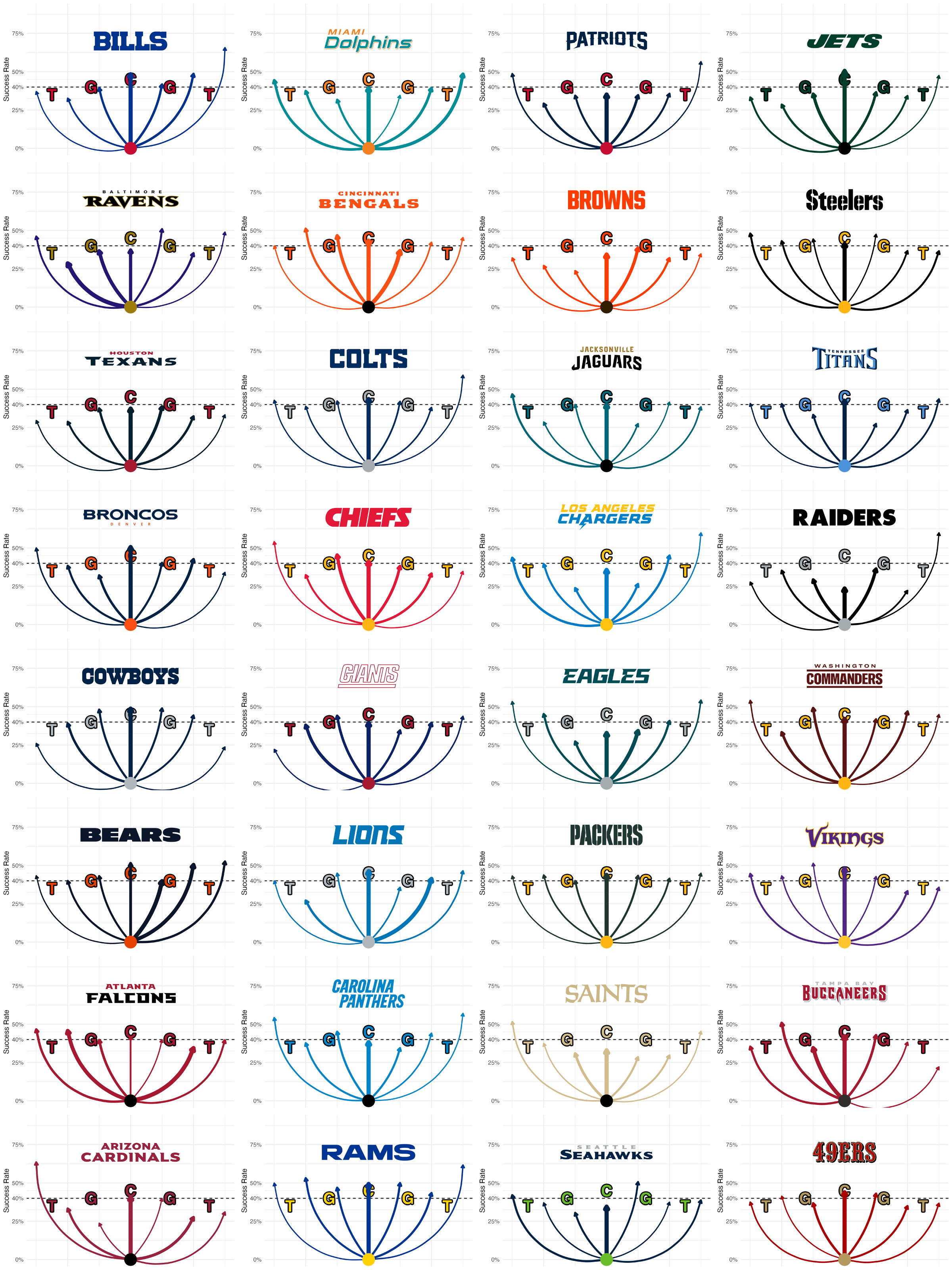
To see this visualization at work, I have created a chart for all 32 NFL teams' rushing success by gap and location for the 2025 season, seen below.
-
The Chicago Bears' rushing attack came alive under Ben Johnson, especially behind Right Tackle Darnell Wright.
Chicago boasted a success rate greater than 50% in three categories, two of which were heavily influenced by Wright's ability to push defenders downfield. Rookie head coach Ben Johnson was hailed as an expert in running the football during his time with the Detroit Lions, and after his first year things seem to be clicking quickly for the team's rushing offense. -
It takes more than just a talented RB to run the ball well, especially up the middle.
After selecting Heisman Trophy finalist Ashton Jeanty sixth overall in the 2025 draft, the Las Vegas Raiders' rushing attack was abysmal, with a league-worst success rate on runs up the middle of 23.6%. The explosive back made up for the disappointment on the outside, but improvements will certainly need to be made to the team's interior offensive line heading into 2026 in order for some positive regression to emerge.
There are many more applications for this tool that I could write analyses of as well. For instance, we can isolate by the player rather than the team to see how backs in the same situation compare. Furthermore, we can analyze year-over-year regression on the same team to understand how they improved or deteriorated over time. Alternative implementations such as these can be found in the source code for this project.
The Code
If you would like to learn more about this project, you may view and download the code for yourself using the button below. Thanks for reading!